Ask a Bayesian: Who Is Better at Wordle?

Just want to compare two players? Check out the accompanying DeepNote notebook. To keep up with our writing, sign up for our newsletter and follow us on Twitter!

I’ve played through 80-something games of Wordle. I’m not bad at it: I’ve been able to guess every word correctly (so far), and I finish in three to five guesses most of the time. It takes me 3.88 guesses, on average, to get the correct word.

My friend started playing Wordle just a few weeks ago. They’ve logged sixteen games and have had some serious beginner’s luck, with an average of 3.45 guesses per round (figure 1). They even got the right word on the first guess once.

Now they’re convinced they’re the better Wordle player. I disagree. In this post, I will conduct a Bayesian analysis of our scores in order to make my case. I will find out who’s better at Wordle, and, more importantly, I will show how to reason about uncertainty like a Bayesian.

Figure 1: I have played many more games than my friend, but my friend has a better (lower) average number of guesses per round.

Bayesian Analysis of the Difference between Scores

To figure out who is better, we need a metric for skill at Wordle. We will use the average number of guesses per round as a proxy for Wordle skill. At this point, you might ask, isn’t the analysis over? After all, my friend has the better average number of guesses, so they’re the better better player, right?

Suppose my friend had only ever played one game, and they finished in four guesses. Would we then conclude that they are worse, based on one data point? Of course not! We need more data. Even after sixteen games, we’re a lot less confident about their skill at Wordle than we are about mine. A couple of bad games could change their average quite a bit, while it would take a lot more games to meaningfully change my average.

Bayesian analysis gives us the tools to estimate metrics of interest, such as Wordle skill as measured by the average number of guesses per round, and to measure the uncertainty surrounding those metrics. Only by modeling the uncertainty in our respective averages can I show that I might be the better Wordle player.

Of course, Bayesian methods aren’t the only tools at our disposal. For a gentle introduction to Bayesian thinking and a comparison to the other major statistical tradition, Frequentist statistics, see the documentation for the bayestestR package, which we used in this analysis. We chose the Bayesian approach for this analysis because of its interpretability: the results can be described in terms of simple probabilities without reference to imaginary repeated experiments, as is often required by Frequentist methods.

Steps in Bayesian analysis

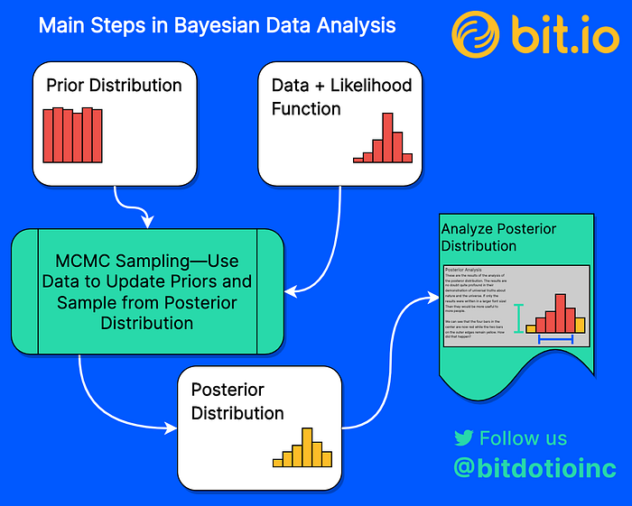
There are three key steps to Bayesian inference:

1. First, we choose a prior distribution. The prior is a statistical distribution that expresses our belief about the probability of winning a round of Wordle in N guesses, where N is an integer between 1 and 6.
2. Second, we choose a likelihood function. The role of the likelihood function is to describe how the probabilities of winning a round in each number of guesses relate to the observed data, the actual number of games won in each of one through six guesses for both me and my friend.
3. Lastly, we update our prior beliefs about the probabilities of completing a round in N guesses based on the observed data, resulting in a posterior distribution. The posterior balances our prior beliefs and knowledge against what we learn from the data. If we have strong prior knowledge and limited data, the posterior will resemble the prior. If we have weaker prior knowledge and plenty of data, the posterior will more closely resemble the data distribution. We sample from the posterior distribution using a process called Markov Chain Monte Carlo Sampling.

Figure 2: The main steps in Bayesian data analysis. We first specify the prior and likelihood, and then use Markov Chain Monte Carlo methods to sample from the posterior distribution. To draw inferences, we analyze the posterior distribution itself.

The key point to remember is that the prior represents the model’s beliefs before it has seen any data while the posterior represents the model’s beliefs after seeing the data. Some argue that the Bayesian approach of using prior beliefs allows our subjective assumptions to enter the model. However, all statistical models involve some assumptions; one of the benefits of the Bayesian approach is that it requires us to make them clear and explicit.

See the technical notes at the bottom for some more details and for the JAGS model. Figure 3 shows the prior and posterior distributions of the probabilities of finishing a round of Wordle in N guesses.

Figure 3: The prior distribution doesn’t make any strong assumptions about the probability of finishing a round of Wordle in any given number of guesses (1–6).

There are a few key observations about how we chose to model the data:

• We want the model to be completely agnostic to play style, so we use a relatively weak and uninformative prior. In other words, we’re making our ignorance about the underlying probabilities an explicit part of the model.
• The prior probability distribution for each number of guesses and for each player are the same. The prior distribution is not based on any data, so there are no differences (outside of sampling variability). In particular, the mean of the prior distribution for each number of guesses is about ⅙, which implies that we make no assumptions that any number of guesses is more probable than any others.
• In the posterior distribution, my probabilities tend to be more concentrated than my friend’s. This is because I’ve played many more rounds. The model has more data to work with, so the vague prior has little impact on the posterior distribution while the data are much more impactful. My friend has played fewer games, though, so the prior will have more influence.

See the “Technical Notes” section at the end for more details about the modeling process.

It bears repeating that both the prior and the posterior are distributions, not single values. We can estimate the “most plausible” estimates by taking, for example, the mean or mode of the distribution. But we use the whole distribution to understand the uncertainty around each estimate.

So, Who’s Better?

Using the distributions of probabilities, we can compute the distribution of the average number of guesses for each player, and the distribution of the difference between our scores (figure 4). A player’s mean score is just the weighted average of each number of guesses (one through six) with the corresponding posterior probabilities. Doing this for both players and taking the difference between the two scores gives the difference. We can then analyze the posterior mean scores and the posterior difference.

Figure 4: The prior distributions of our average numbers of guesses are roughly the same. Before seeing the data, the model does not suggest that either of us is the better player, as it has not yet seen any data. The posterior, on the other hand, shows high confidence that my average guess number is just under 4, and somewhat less confidence that my friend’s average guess number is closer to 3.5.

Understanding Uncertainty

Figure 4 shows why we really need to care about uncertainty. Given their 16 games, the most plausible values for my friend’s average number of guesses per round are better than mine–but there’s a lot of uncertainty. The distribution of their average number of guesses has much heavier tails than mine, meaning that the model is a lot less certain about their average. Their average guess number falls between 2.94 and 4.10 with 95% probability: a wide range.

My posterior average guess number, on the other hand, sharply peaked around 3.86 with very narrow tails. My average guess number falls between 3.66 and 4.07 with 95% probability. This range is fully included in my friend’s range, meaning that it’s possible they’re better, the same, or even worse than I am at Wordle.

To get a more precise idea, let’s look at the posterior distribution of the difference between our average scores.

Figure 5: The prior distribution of our differences in scores is approximately 0 (approximate because of variability from the sampling procedure), which makes sense given the nearly-identical prior distributions of our averages shown in figure 4. The posterior, however, is around 0.36 because my friend’s average score is better than mine. But there is still plenty of uncertainty: it is unlikely, but far from impossible, that our Wordle skills are the same, or even that I’m the better player.

Most of the probability density shows a difference in our scores greater than zero, suggesting that my friend is, indeed, a better Wordle player than I am. The 95% highest density interval (HDI) for the difference is -0.25 to 0.98 guesses: a wide range that includes zero, leaving open the possibility that our Wordle skills are equal (or close to it).

How certain are we? Well, about 75% of the posterior density for the difference is greater than zero, translating to a 75% posterior probability that my friend is the better Wordle player, as measured by the average number of guesses to win a round. While this won’t clear the (arbitrary) bar of a p-value of 0.05, it is highly suggestive.

In other words, I need to improve my Wordle game!

Want to read more like this? Sign up for our newsletter and follow us on Twitter!

Technical Notes

We used a Dirichlet prior with a concentration parameter of 1, and we modeled the data with a Multinomial likelihood function. This results in a Dirichlet-Multinomial posterior distribution. We used JAGS (Just Another Gibbs Sampler) to sample from the prior and posterior distributions and to estimate the average numbers of guesses and the differences between averages.

The JAGS model (as implemented in R) is as follows:

To experiment with different priors (or entirely different models), make a copy of the Deepnote notebook and edit the model. You might, for example, try to specify a Dirichlet prior that places a very low probability on guessing correctly on the first guess by making alpha a vector.